Tree Traversal

Traversals

Trees are an essential part of storing data, or at computer scientists like to refer them as, data structures. Among their benefits is that they’re optimized to be searchable. Occasionally you need to serialize the entire tree into a flat data structure. Today we’ll show you how to do that.

^{Public domain, via Wikimedia Commons}

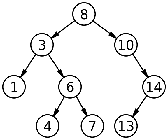
The picture tree is a valid binary search tree (BST.) We’re going to show you four different ways serialization of this BST: three variations of depth-first traversal and one that is breadth-first traversal.

Depth-first Traversal

Let’s start with one variant depth-first traversals: pre-order traversal. The basic gist is that for each of the nodes, you process the node (in our case, save it to an array since we’re serializing this tree,) then process the left subtree and then the right tree. Let’s write out that works.

Given the above tree:

text
-> Call our method (let's call it preorderTraverse) on the root node, 8.
-> Add 8 to our array.
-> Call preorderTraverse on the left child, 3.
-> Add 3 to our array.
-> Call preorderTraverse on the left child, 1.
-> Add 1 to our array.
-> Has no children, returns.
-> Going back up the tree, we'll call preorderTraverse on 6.
-> Add 6 to our array.
-> Call preorderTraverse on the left child, 4.
-> Add 4 to our array.
-> No children, returns.
-> Going back up the tree, we'll call preorderTraverse on 7.
-> Add 7 to the array.
-> So on and so forth.

We end up with the array of [8, 3, 1, 6, 4, 7, 10, 14, 13]. This is called preorder traversal.

The other variants are quite similar; the only thing we do is change the order. When I say “process the node,” I mean you do whatever operation you’re going to do: add it to an array, copy the node, or whatever that may be.

In preorder traversal, you process the node, then recursively call the method on the left subtree and then the right subtree.

In inorder traversal, you first recursively call the method on the left tree, then process the node, and then call the method on the right tree.

Postorder traversal, as you have guessed, you recursively call the method on the left subtree, then the left subtree, then you process the node. The results of these are as follows:

text
// preorder
[8, 3, 1, 6, 4, 7, 10, 14, 13]
// inorder
[1, 3, 5, 6, 7, 8, 10, 13, 14]
// postorder
[1, 4, 7, 6, 3, 13, 14, 10, 8]

As you can see, it depends on what you’re doing on which of these you use. For a sorted list out of a BST, you’d want to use inorder. If you’re making a deep copy of a tree, preorder traversal is super useful since you’d copy a node, and then add its left child and then its right tree. Postorder would be useful if you’re deleting a tree since you’d process the left tree, then the right, and only after the children had been deleted would you delete the node you’re working on.

So let’s go give this a shot!

Exercises

Breath-first Traversal

Now that you’ve done depth-first, let’s tackle breadth-first. Breadth-first isn’t recursive processing of subtrees like depth-first. Instead we want to process one layer at a time. Using the tree above, we want the resulting order to [8, 3, 10, 1, 6, 14, 4, 7, 13]. In other words, we start at the root, and slowly make our way “down” the tree.

The way we accomplish this is using our old friend, the queue. A queue is an array that the first thing you into is the first thing you get out of it (FIFO, first in first out, as opposed a stack which is first in last out, FILO.) Another way of thinking about it is that if you call dequeue on a queue, the item that has been in there the longest is the one that comes out.

What we’re going to do is process the node, then add the left child to the queue and then add the right child to the queue. After that, we’ll just dequeue an item off of the queue and call our function recursively on that node. You keep going until there’s no items left in the queue.

Let’s do the exercise! This can be solved recursively or iteratively, with the iterative result being the preferred of the two.

text
-> start function by adding root to the queue, queue = [8]
-> process 8, add to final array array = [8]
-> queue 3 and 10 to queue, queue = [3, 10]
-> dequeue 3, queue = [10]
-> queue 3's children, queue = [10, 1, 6]
-> add 3 to final array, array = [8, 3]
-> dequeue 10, queue = [1, 6]
-> queue 10's children, queue = [1, 6, 14]
-> add 10 to final array, array = [8, 3, 10]
-> dequeue 1, queue = [6, 14]
-> queue 1's children, nothing
-> add 1 to final array, [8, 3, 10, 1]
[etc.]
final array is [8, 3, 10, 1, 6, 14, 4, 7, 13]

So why is this useful? This is really useful if you’re looking for something you know is going to be near the root of the tree or if you’re looking for the “closest” (e.g. least hops) node to something. For example, if your tree represents a social network and you’re looking to recommend to them who to follow, you might do a breadth-first traversal of their social contacts and recommend them people with 2 degrees of separation. Breadth-first traversal is perfect for that.

Breadth-first traversals are useful for many things and we’ll be using the algorithm when we do path-finding, but the gist of when you use them is that you know the answer for what you’re looking for is “closer” to the root node as opposed to far away when you would use depth-first. Again, it’s all trade-offs and what you’re trying to do.

Exercises